Convolutional neural net Part 3 Downsampling
- last_theorem
- May 16, 2021
- 3 min read
Updated: Oct 24, 2021
The main idea of the pooling/stride operation is the compression of the image data. Remember I mentioned one of the most fundamental problems solved by the convolutions neural net is, it captures the high level and the low-level features. So how is this done, the low-level features are captured in the first few layers of the convolution network, as the network gets denser, it introduces several pooling operations to the image, which compress the image data. When you commit several rounds of pooling operation on the image data the image starts to shrink trying to maintain the high-level features, and at this high-level features are observed by the network. The pooling operation also helps in downsampling the image and try to show the dominating pixels. So when this downsampling happens by the polling operation, it makes sure that the most relevant informations are preserved.

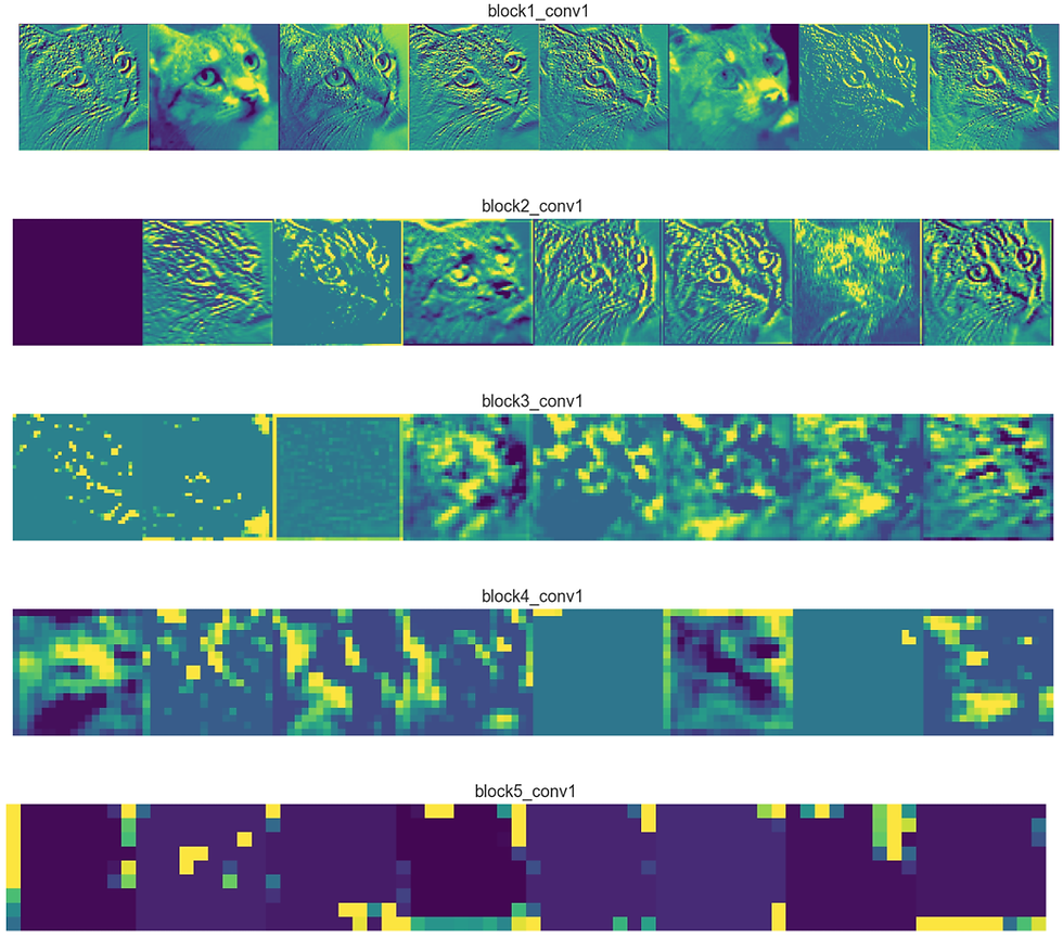
Fig:1 Here you can what a pooling operation does to the image, as the layer progress forward the pooling operation compresses the images. So the conv layer at the bottom looks at the high-level features of the image.
What are the different kinds of pooling operations?
MaxPooling
The idea of the max-pooling is to take the maximum number from a grid of pixels. Why do we do this, we are simply picking the most dominating pixel. This process of pooling is a downsampling process. When you repeated this process several times we end up with a set of pixels that dominated the image.
import matplotlib.pyplot as plt
from matplotlib import image

file_path=r"D:\Google Drive\File transfer_\IMG_20190530_091107__02.jpg"
data = image.imread(file_path)
plt.imshow(data)
image = data.reshape(1, 1589, 1147, 3)

for x in range(6):
    model = Sequential()
    for y in range(x):
        model.add(MaxPooling2D(pool_size = 2, strides = 2))
    # generate pooled output
    output = model.predict(image)
    array.append(output)


#creating a subplot
fig,ax =  plt.subplots(1,6)
fig.set_figheight(5)
fig.set_figwidth(20)
count=0
x=list(range(1,110,10))
for row in range(ax.shape[0]):
        img=np.squeeze(array[count])
        ax[row].imshow(img)
        count=count+1
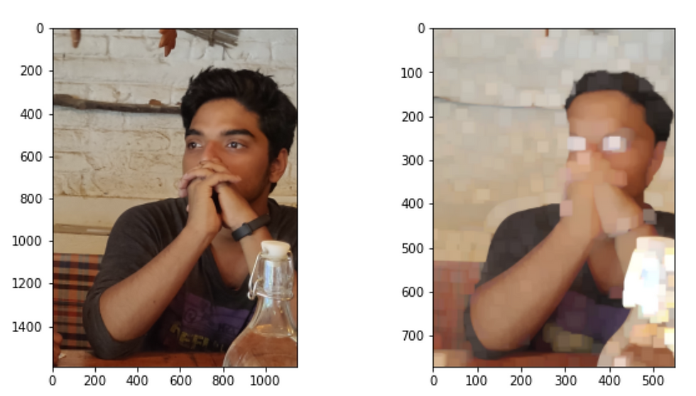
Fig:2 (output of above code )This is an example of the max pooling operation, the pixels which dominate the image are popping out and providing a high-level view of the image. This is the idea of the pooling operation.

Fig:3
This is what is happening internally, the max-pooling operation is picking the maximum number from an image grid. Here in this case we are using a max pooling function from the keras, and 2d window is used in size set 2 (very much like the fig above). So this operation is repeated consistently to downsample the image. As you can see from Fig:2 how the image is shrinking in its size.
Average pooling
In the case of the average pooling involves calculating the average for each patch of the feature map. This means that each 2×2 square of the feature map is downsampled to the average value in the square. This work very much like the max-pooling, but in the case of avg pooling, we consider the average of the feature map instead of the maximum.

Fig:4
from keras.layers import AveragePooling2D
array_avg=[]
image = data.reshape(1, 1589, 1147, 3)

for x in range(6):
    model_ = Sequential()
    for y in range(x):
        model_.add(AveragePooling2D(pool_size = 2, strides = 2))
    # generate pooled output
    output = model_.predict(image.astype('float64'))
    array_avg.append(output)


#creating a subplot
fig,ax =  plt.subplots(1,6)
fig.set_figheight(5)
fig.set_figwidth(20)
count=0
x=list(range(1,110,10))
for row in range(ax.shape[0]):
        img=np.squeeze(array_avg[count])
        ax[row].imshow(img.astype("int64"))
        count=count+1
Fig:5
Output of the average pooling
Global Pooling Layers
Instead of downsampling patches of the input feature map, global pooling downsamples the entire feature map to a single value. This would be the same as setting the pool_size to the size of the input feature map.
Global pooling can be used in a model to aggressively summarize the presence of a feature in an image. It is also sometimes used in models as an alternative to using a fully connected layer to transition from feature maps to an output prediction for the model.
Stride


Stride is another way of down sampling the image data. This is simply offset of convolutional window to down sample the image. In the about image you have the stride value 1 , so there is only 1 pixel difference between the first convolutoinal window and second one . You can think about this as how much distance you need in between the convolutional window placement.
from keras.layers import AveragePooling2D
array_avg=[]
image = data.reshape(1, 1589, 1147, 3)

for x in range(6):
    model_ = Sequential()
    for y in range(x):
        model_.add(AveragePooling2D(pool_size = 2, strides = 4))
    # generate pooled output
    output = model_.predict(image.astype('float64'))
    array_avg.append(output)


#creating a subplot
fig,ax =  plt.subplots(1,6)
fig.set_figheight(5)
fig.set_figwidth(20)
count=0
x=list(range(1,110,10))
for row in range(ax.shape[0]):
        img=np.squeeze(array_avg[count])
        ax[row].imshow(img.astype("int64"))
        count=count+1
This is a visual context of how the stride down sample the images , some times you need multiple pooling layer to capture the high level details, with stride this can be done with few layers . There should a balance maintained on how much data should be preserved and how much you need to maintain for better capturing of features. Thus stride also become a hyper parameter.

コメント