Convolutional neural net Part 4 Full picture
- last_theorem
- May 16, 2021
- 7 min read
Updated: Oct 24, 2021
Until now we focused on some basic concepts from the convolutional network, now we are about to look, how these all ideas work together to build a great mechanism to handle the image data. I already mentioned some of the computer vision problems on features and how the algorithm should look into high and low-level features to understand the image data. With the convolution we can solve this problem, the initial version was not the ideal one but later with several iterations we managed to build CNNs with much better accuracy. Here we are going to see how.
How does the convolutional network work?
What is a Convolution window?
By this time, We have a reasonably good understanding of some of the founding ideas in the convolutional neural net.
We know that this network looks at the high-level and low-level details of an image.
This is done with the help of
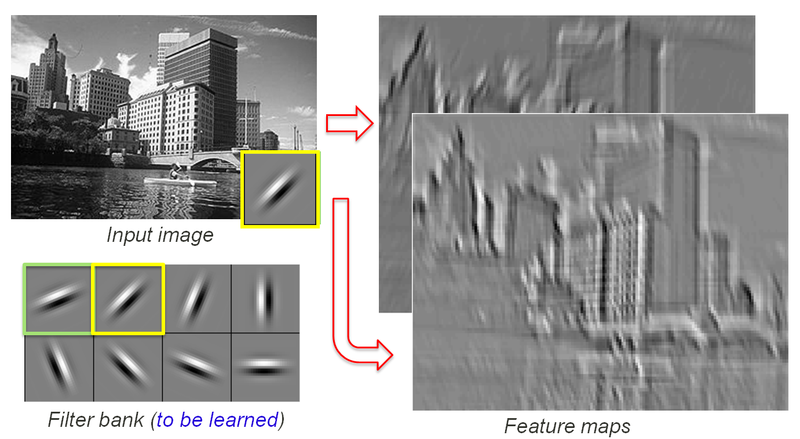
Kernels /Filters, kernel is used to pick up the features
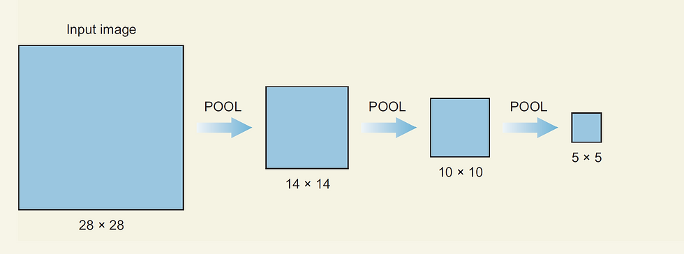
Pooling operations. , is a compression technique used to see the high-level features of the image, Also this a very effective compression/down-sampling mechanism.
The next question would be, how do we implement this idea to an input image, is it like we have a 128x 128-pixel image as input and we directly put a kernel on it and then do multiple pooling operations. It turns out. One of the reasons for that is we drastically lose a lot of information from image data, this could make us almost impossible to solve problems like object detection which is very sensitive to features.
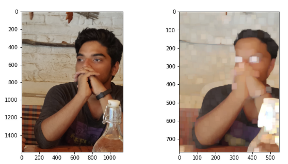
Fig:1
(This is a visual context of what would happen if you don’t use a larger convolutions window(50,50). If we don’t use a convolutional window and directly use a max-pooling then we will shrink to a single value and the purpose will be lost. )
We have a very effective way of doing both this operation on an image input. This method can serve all our purpose,
Collecting the image features from low level to high level.
Reduce the data loss.
Implement the kernels for capturing the features.
It's called convolution windows, the convolutional neural network gets its name from this idea of convoluting windows.
Fig:2 (A convolutional window is basically grid or window of the matrix which loop or convolutes through the image input. The gif and the image will provide you a visual context of what is mean by this convolutional window.)
Fig:3
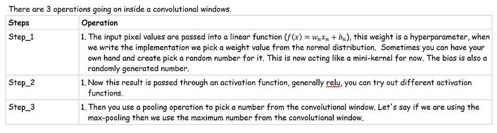

Fig:4
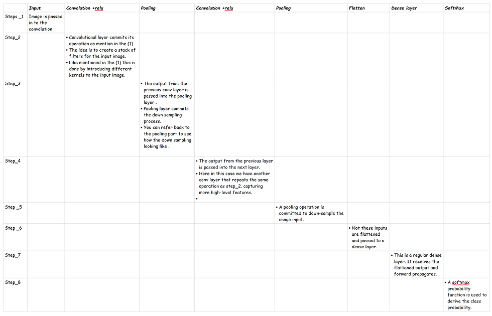
The Fig:4 is giving you a visual context to what happens inside a convolutional window.
It applies the filter
Then it's passed through an activation filter
The resulted filter from 1 and 2 is further passed into a pooling layer which downsamples the filter.
Step no 1,2 is repeated several times very much as shown in Fig:2. The convolutional window convolutes throughout the image. You can imagine this as like a scanner looping through an image. And produces multiple filters of the same image. (As I mentioned its not hard to create a filter, you just need to randomly assign a weight and bias to the input pixel value) . In a convolutional neural net, we repeat this process multiple times and create such multiple filters sometimes 256, 128 etc.
The number of filters you need to create depends on what kind of network you need to build, the depth of the network, the number of kernels used, how you are stacking each of these networks what defines a convolutional neural net. In a search result, you will find different types of neural nets all these nets simply differ in how they are configured. The fundamental of all these networks remains same.
Padding
These are two configurations you need to understand in the convolutional window. Look at Fig :5 . There you can see, the convolutional window is not fit properly on the image as you see in Fig:2 . Now, this is a problem, after all, we are working with a mathematical problem here. So the question is how do we solve this . ?
It turns out you can add some empty pixels into it, very much like a border, and it's called padding. So padding is simply some border space for the image.
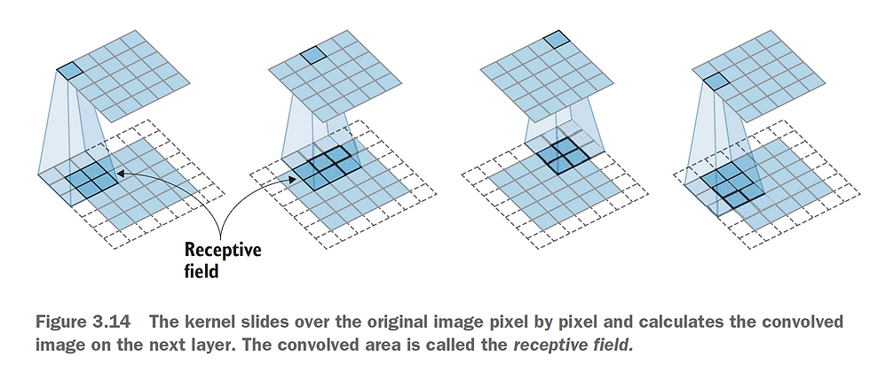
Fig:5 the white border around the image is the padding.
Going further

As you can see here, there are 4 kernels created from the input image, and this is passed to the next layer. The next layer(28,28,4) also runs a similar operation on each of the kernels and creates another (28,28,12) filter. One thing to notice here is we haven't introduced any pooling layer in this, if we introduce a pooling layer then we can compress/downsample the image in a much smaller dimension. These compression filters could help the network to look into the high-level features.
What is the full picture like?

The kernel size is a hyperparameter, the user can decide how many kernels each of the conv layers should generate.
If you are following some standard networks like vgg, retinet etc follow the same configuration.

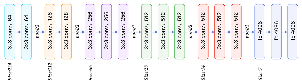
This is a look into the vgg16 architecture. As you can see here, how the network is stacked, the number of filters used to capture features, the points where max-pooling layer is introduced.
What happens during backpropagation?
We are not going to get into the very details of how does the backpropagation work in the case of CNN in every detail. Rather we will be provided with some high-level view about the idea and what basically happens in CNN. The entire idea of the backpropagation algorithm is to adjust the weights and the biases to reduce the loss function. This remains same for the CNN as well. The idea is to readjust the weights of all the kernels. Which I mentioned in the step_1 (convolutional windows) . Think back to the concepts of kernels I introduced in the previous blog. How kernels are used to do certain operations on the image data. Here we are going to use the kernels to absorb the features in the image. And this is done by adjusting the weights in the kernels. This adjustment is done by the backpropagation algorithm.
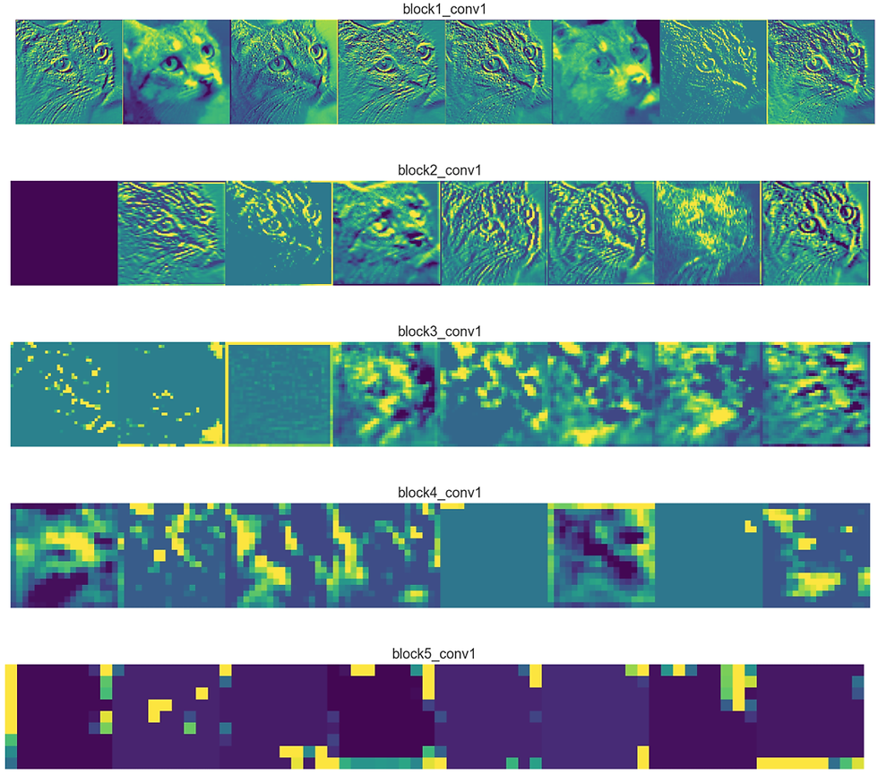
These are some inside images from the filters, this is how the filters looks like after the training process is over. Now get into google do some image search on visualization of feature maps, you will find a whole lot of information about this . Now in a fully trained CNN, when you input an image the trained weights and biases will pick up those trained features and the activation will be fired accordingly and proceeds to the next layer and this operation is repeated until the last layer.
Implementation
Let's have a look at how the implementation really works, we are going to use TensorFlow version 1 for this purpose, this is a very low-level implementation of the convolutional neural nets , now we don’t depend on this kind of implementation to build a larger network rather we use high-level implementations. This entire example is to give you an idea how these theories we have learned combine together to form a neural net.
I want to start with the most high-level implementation with Keras , we will move into a low-level implementation as well. Please check both of the implementations. In case if this code doesn't in your device. Download the notebook and check again.
import numpy as np
from tensorflow import keras
from tensorflow.keras import layers

# Model / data parameters
num_classes = 10
input_shape = (28, 28, 1)

# the data, split between train and test sets
(x_train, y_train), (x_test, y_test) = keras.datasets.mnist.load_data()

# Scale images to the [0, 1] range
x_train = x_train.astype("float32") / 255
x_test = x_test.astype("float32") / 255
# Make sure images have shape (28, 28, 1)
x_train = np.expand_dims(x_train, -1)
x_test = np.expand_dims(x_test, -1)
print("x_train shape:", x_train.shape)
print(x_train.shape[0], "train samples")
print(x_test.shape[0], "test samples")


# convert class vectors to binary class matrices
y_train = keras.utils.to_categorical(y_train, num_classes)
y_test = keras.utils.to_categorical(y_test, num_classes)

model = keras.Sequential(
    [
        keras.Input(shape=input_shape),
        layers.Conv2D(32, kernel_size=(3, 3), activation="relu"),
        layers.MaxPooling2D(pool_size=(2, 2)),
        layers.Conv2D(64, kernel_size=(3, 3), activation="relu"),
        layers.MaxPooling2D(pool_size=(2, 2)),
        layers.Flatten(),
        layers.Dropout(0.5),
        layers.Dense(num_classes, activation="softmax"),
    ]
)

model.summary()

batch_size = 128
epochs = 15

model.compile(loss="categorical_crossentropy", optimizer="adam", metrics=["accuracy"])

model.fit(x_train, y_train, batch_size=batch_size, epochs=epochs, validation_split=0.1)

score = model.evaluate(x_test, y_test, verbose=0)
print("Test loss:", score[0])
print("Test accuracy:", score[1])
Tensorflow Implementation
#importing the dependency
import numpy as np
import matplotlib.pyplot as plt
import tensorflow as tf
z
from sklearn.model_selection import train_test_split

from numpy import asarray
from keras.models import Sequential
from keras.layers import Conv2D

from six.moves import urllib
import tarfile
import os

from sklearn import datasets
digits = datasets.load_digits()


# Load in the data
mnist = tf.keras.datasets.mnist

(x_train, y_train), (x_test, y_test) = mnist.load_data()
x_train, x_test = x_train / 255.0, x_test / 255.0
print("x_train.shape:", x_train.shape)

train_dataset=tf.data.Dataset.from_tensor_slices((x_train,y_train)).batch(20)
testing_dataset=tf.data.Dataset.from_tensor_slices((x_test,y_test)).batch(20)


num_channel=1
image_height=x_train.shape[1]
image_width=x_train.shape[2]
target_size=np.max(y_train) + 1
batch_size=100
evaluation_size=500
generations=500
conv1feature=25
conv2feature=50
max_pool_size1=2
max_pool_size2 =2
fully_connected_size1 =100
learning_rate = 0.005
eval_every =5

#creating the placeholder
x_input_shape=(batch_size,image_width,image_height,num_channel)

x_input =tf.compat.v1.placeholder(tf.float32,shape=x_input_shape)
y_target=tf.compat.v1.placeholder(tf.int32,shape=batch_size)

#creating placeholder for evaluation
eval_input_shape = (evaluation_size, image_width, image_height,num_channel)

eval_input = tf.compat.v1.placeholder(tf.float32, shape=eval_input_shape)
eval_target =tf.compat.v1.placeholder(tf.int32, shape=(evaluation_size))


#declaring the convolutional weight
conv1weight=tf.Variable(tf.random.truncated_normal([4,4,num_channel,conv1feature],stddev=0.1,dtype=tf.float32))
conv2weight=tf.Variable(tf.random.truncated_normal([4,4,num_channel,conv2feature],stddev=0.1,dtype=tf.float32))

conv1bias=tf.Variable(tf.zeros([conv1feature]),dtype=tf.float32)
conv2bias=tf.Variable(tf.zeros([conv2feature]),dtype=tf.float32)


#conncting the weights and the biases.
"""This is the resulting size after the convolutional operation ."""
resulting_width=image_width // (max_pool_size1 * max_pool_size2)
resulting_height=image_height // (max_pool_size1 * max_pool_size2)
full1_input_size=resulting_width*resulting_height*conv2feature

full1_bias= tf.Variable(tf.random.truncated_normal([fully_connected_size1]) )
full2_bias= tf.Variable(tf.random.truncated_normal([target_size],stddev=0.1, dtype=tf.float32) )
full2_weight= tf.Variable(tf.random.truncated_normal([fully_connected_size1,target_size],stddev=0.1, dtype=tf.float32) )
full1_weight= tf.Variable(tf.random.truncated_normal([full1_input_size, fully_connected_size1],stddev=0.1, dtype=tf.float32) )


#initializing the model operation
def my_conv_net(inputdata):
  #first conv relu- max pooling layer
  conv1=tf.nn.conv2d(inputdata,conv1weight,strides=[1,1,1,1],padding="SAME")
  relu1=tf.nn.relu(tf.nn.bias_add(conv1,conv1bias))
  max_pooling1=tf.nn.max_pool(relu1,ksize=[1,max_pool_size1,max_pool_size1,1],strides=[1, max_pool_size1, max_pool_size1, 1],padding="SAME")

  #second conv ,relu, max-pool layer
  conv2=tf.nn.conv2d(max_pooling1,conv2weight,strides=[1,1,1,1],padding="SAME")
  relu2=tf.nn.relu(tf.nn.bias_add(conv2,conv2bias))
  max_pooling2=tf.nn.max_pool(relu2,ksize=[1,max_pool_size2,max_pool_size2,1],strides=[1, max_pool_size2, max_pool_size2, 1],padding="SAME")

  # Transform Output into a 1xN layer for next fully connected layer
  final_conv_shape=max_pooling2.get_shape().as_list()
  final_shape =final_conv_shape[1]*final_conv_shape[2]*final_conv_shape[3]
  flat_output=tf.reshape(max_pooling2,[final_conv_shape[0],final_shape])

  # First Fully Connected Layer
  fully_connected1 =tf.nn.relu(tf.math.add(tf.linalg.matmul(flat_output ,full1_weight),full1_bias))

  #second fully connected model
  final_model_output =tf.nn.relu(tf.math.add(tf.linalg.matmul(fully_connected1,full2_weight),full2_bias))

  return final_model_output


#creating the model
model_output = my_conv_net(x_input)
test_model_output = my_conv_net(eval_input)


#creating the loss function
loss = tf.reduce_mean(tf.nn.sparse_softmax_cross_entropy_with_logits(logits=model_output,labels=y_target))


# Create a prediction function
prediction = tf.nn.softmax(model_output)
test_prediction = tf.nn.softmax(test_model_output)

#creating a accuracy function
def get_accuracy(logits,target):
  batch_predictions=np.argmax(logits,axis=1)
  num_correct= np.sum(np.equal(batch_predictions,target))
  return (100*num_correct/batch_predictions.shape[0])


#creating optimizer
my_optimizer = tf.compat.v1.train.MomentumOptimizer(learning_rate,.9)
trainining_step = my_optimizer.minimize(loss)


# Start training loop
train_loss = []
train_acc = []
test_acc = []
# sess=tf.compat.v1.Session
with tf.compat.v1.Session()  as sess:
  init = tf.compat.v1.global_variables_initializer()
  sess.run(init)

  for x in range(generations):
    rand_index= np.random.choice(len(x_train),size=batch_size)
    rand_x=x_train[rand_index]
    rand_x=np.expand_dims(rand_x,3)
    rand_y= y_train[rand_index]
    train_dic= {x_input:rand_x,y_target:rand_y}

    #Calling the session
    sess.run(trainining_step,feed_dict=train_dic)

    temp_train_loss, temp_train_preds =  sess.run([loss,prediction],feed_dict=train_dic)
    temp_train_acc = get_accuracy(temp_train_preds, rand_y)

    if (x+1) % eval_every ==0:
        eval_index = np.random.choice(len(x_test), size=evaluation_size)
        eval_x = x_test[eval_index]
        eval_x = np.expand_dims(eval_x, 3)
        eval_y = y_test[eval_index]
        test_dict = {eval_input: eval_x, eval_target: eval_y}
        test_preds = sess.run(test_prediction, feed_dict=test_dict)
        temp_test_acc = get_accuracy(test_preds, eval_y)

         # Record and print results
        train_loss.append(temp_train_loss)
        train_acc.append(temp_train_acc)
        test_acc.append(temp_test_acc)
        acc_and_loss = [(x+1), temp_train_loss, temp_train_acc, temp_test_acc]
        acc_and_loss = [np.round(x,2) for x in acc_and_loss]
        print('Generation # {}. Train Loss: {:.2f}. Train Acc (Test Acc): {:.2f} ({:.2f})'.format(*acc_and_loss))


# Matlotlib code to plot the loss and accuracies
eval_indices = range(0, generations, eval_every)
# Plot loss over time
plt.plot(eval_indices, train_loss, 'k-')
plt.title('Softmax Loss per Generation')
plt.xlabel('Generation')
plt.ylabel('Softmax Loss')
plt.show()

# Plot train and test accuracy
plt.plot(eval_indices, train_acc, 'k-', label='Train Set Accuracy')
plt.plot(eval_indices, test_acc, 'r--', label='Test Set Accuracy')
plt.title('Train and Test Accuracy')
plt.xlabel('Generation')
plt.ylabel('Accuracy')
plt.legend(loc='lower right')
plt.show()


# Plot some samples
# Plot the 6 of the last batch results:
actuals = rand_y[0:6]
predictions = np.argmax(temp_train_preds,axis=1)[0:6]
images = np.squeeze(rand_x[0:6])

Nrows = 2
Ncols = 3
for i in range(6):
    plt.subplot(Nrows, Ncols, i+1)
    plt.imshow(np.reshape(images[i], [28,28]), cmap='Greys_r')
    plt.title('Actual: ' + str(actuals[i]) + ' Pred: ' + str(predictions[i]),
                               fontsize=10)
    frame = plt.gca()
    frame.axes.get_xaxis().set_visible(False)
    frame.axes.get_yaxis().set_visible(False)
plt.show()
Download the notebook from the below link:


Comentarii