Read Me
The objective of this blog is not to transform you into a proficient coder or programmer overnight. Instead, it aims to provide you with threads that will help develop your skills and broaden your perspective as a beginner. When I initially drafted the blog and shared it with some of my peers (who are some professional programmers) , they cautioned me that I might be overly ambitious. They pointed out that expecting readers to fully grasp each concept presented, especially considering that each concept requires an in-depth explanation of around 8,000 words, might be unrealistic. Therefore, it's essential to keep in mind that there's considerable depth and nuance to each segment. If you find yourself struggling with a particular section, it's important to pause, conduct additional research, and then continue your reading journey.
Introduction
Programming has come a long way since its inception, and one of the major milestones in its evolution was the introduction of object-oriented programming (OOP). Before OOP, programming was primarily done using procedural programming languages, which had their own set of advantages and limitations. In this essay, we will explore how programming was before the advent of OOP, why it needed a paradigm shift, where it was used, and how it has transformed the way software is developed.
What is Procedural Programming?
Procedural programming is a programming paradigm that focuses on creating procedures or routines to perform specific tasks. It revolves around breaking down a program into smaller functions or procedures that can be executed sequentially. These procedures manipulate data by altering their values or passing them as arguments between different functions. Object-oriented programming (OOP) emerged as a solution to the limitations of procedural programming. It introduced a new way of organizing and structuring code by focusing on objects rather than procedures.

A computer can only understand binary. In the initial days of computing, the computer instructions (programs) were written on punched tape. These tapes were rolled into a long and sequentially executed. As computing technology advanced, more complex methods were introduced, such as Random Access Memory, which allowed the computers to process the instructions randomly.
As the programming techniques evolved more approaches were introduced to write programs.
Here's an example of a low-level program written in assembly language for the x86 architecture. This program calculates the sum of two numbers and stores the result in a register:
section .data
    num1    db 10        ; first number
    num2    db 20        ; second number

section .text
    global _start

_start:
    mov al, [num1]      ; move first number to AL register
    add al, [num2]     ; add second number to AL register
    mov [result], al   ; store the result in memory location "result"

exit:
    mov eax, 1         ; system call number for exit
    xor ebx, ebx       ; exit status code (0)
    int 0x80           ; invoke the operating system to exit

section .data
    result  db ?        ; uninitialized memory location for storing the result
In this example, we have two numbers `num1` and `num2` defined in the `.data` section. The program starts at `_start` label and moves the value of `num1` to the `AL` register using `mov al, [num1]`. Then it adds the value of `num2` to `AL` using `add al, [num2]`, which modifies the contents of `AL`. Finally, it stores the result in a memory location named `result`.
The program then uses a system call (`int 0x80`) to invoke the operating system and exit with a status code of 0.
As you can observe, the initial days of programming were less readable and involved more steps to execute even a simple operation. This approach is also called low-level implementation, as it makes the programming more abstract.
As the programming methodology evolved, we introduced the idea of object-oriented programming. Through OOP, we were taking a technical shift in programming. At this point, we can write more high-level implementations of computer instructions. What do I mean by high-level and low-level programming? Think about the context of how English grammar works. If I ask you to describe a verb like "walk," it's a very tedious job to do. Instead of describing an action, we pack that piece of information into something called a verb. In the world of computing, we can call this abstraction or a high-level implementation. Something interesting to note in the world of computer science is that the domain as a whole is always leaning towards constant innovation, and the objective is to make things simpler and optimize them for better performance.
What is object-oriented programming? The whole world can be seen through the lens of objects, and each of these objects is interconnected and falls under some kind of hierarchy and is related to some kind of function. Take the example of a car, which is a very good example to understand this concept. A car as a whole can be thought of as an object. If you group a bunch of cars with similar features, then it's called a class of cars or a class of objects. A class refers to a group or category. In the world of any object-oriented programming language, we think about the class first by defining a set of properties associated with the object and building objects from the description provided in the class. Think about this, as we setting the rules of what a specific object we want to design and use the class model to create n number of objects. A while back we were thinking from an object to a class and now we are thinking from a class to an object design. The idea still remains the same a class is referred to as a group , so the code that goes into the class in any programming language based on object oriented approach defines the properties of the object we are trying to design here.
Take a moment and ponder this idea: the entire approach of object-oriented programming is to view the world through the lens of objects. Objects are always associated with certain properties and can be organized into groups.
Let's go back to the example of a car. The whole car is an object. A car has an engine, body, wheels, and seats. If we take the car engine, the engine can also be an object. It has its own properties. Not just the engine, but all the properties associated with it can be considered as individual objects. But for simplicity , let's just consider the engine as an object.
What is happening here is we are wrapping one object inside another object. If you think about it for a while, you'll realize that the whole world can have objects wrapped inside each other. This forms pretty sophisticated relationships. However, this structure of organizing objects provides a beautiful structure for organizing information.
Car class Engine class


Body class

Let's see how does this looks programmatically
# Car class
class Car:
    def __init__(self, color, wheel, seats, engine,roof):
        self._color = color
        self._wheel = wheel
        self._seats = seats
        self._engine = engine
        self.roof= roof
# engine class
class Engine:
    def __init__(self, material, engine_type, no_cyl, cc, rpm):
        self._material = material
        self._engine_type = engine_type
        self._no_cyl = no_cyl
        self._cc = cc
        self._rpm = rpm

# carbody class
class CarBody:
    def __init__(self, body_type, paint_color):
        self._body_type = body_type
        self._paint_color = paint_color
What are datatypes (Dtypes)?
We went one step ahead while framing the classes, but this was necessary to explain the concept. Now, let's unpack that idea. ,Data types. Whatever data input you provide to any programming language is associated with some kind of datatype. Knowing these datatypes is so important because fundamentally, programming is all about data manipulation. When you were creating an object called "car" through defining its properties in a class, you were defining some data fields. We will get into the idea of how we manipulate this data inside the object in a while. What kind of manipulation you can do with a particular object is always associated with its datatype. As someone who writes a program, your awareness about the type of datatype you are working with is basic information.
- There are some primary datatypes in most of the programming languages,
Integer (int)
Like the name suggests it represents any integer value (check the fig 1)
Float (float32 , float64)
The float represents a decimal number, you have 2 varieties in that float 32 and float 64 .
Both of them are two approaches to encoding the decimals, float 64 can accommodate a larger decimal number compared to 32, thus providing more precision. Python by default uses float 64.
Character (Char)
This is a data type used to represent characters, eg: A, B ,C all the alphabet.
Since the world of Python is a much higher implementation than any other language, it doesn't have a character datatype. Instead, it uses strings. I am introducing this concept because I don't want you to wonder at some point if any other programming language returns this datatype as output.
String (str)
A string is a group of characters, when a group of characters combines you have a word, but in our world, it's not necessary that it has to be a word, the string can be a sentence as well, often represented inside " ".

Boolean (bool)
A Boolean is a binary datatype. It returns only two values: true or false. A boolean acts like a switch or is used for binary questions where the answer is either yes or no.
In our specific context, our car class can have a property called a roof, so the car is the one with the roof or without the roof.
Have a look at this example. This is a popular object in the data analytics called series. It enables you to frame 1D data into a data structure called a series. This is done with a constructor called Series. If you check the data type of it, you will see that it is a Series object type. You can dig even deeper into this. The Series stores the 1D array in a property called values. If you check the data type for that, it will be a numpy array. The numpy arrays are very efficient data structures for arrays in Python, and this is done with the help of a library called numpy in Python.


Storage
Now it's time to introduce the idea of storage while covering the objects I mentioned. Programming is all about manipulating values at different levels. When we were defining an object, we were associating the object with its properties. The properties have some datatypes, and some properties can be an object itself. Here, you need to understand how we are storing these properties. There are various ways to store data in any programming language.
Variable
This is the most important and basic approach to storing any data, but why am I saying it's so important? I think the rule to classify something as important or not depends upon the frequency of its usage. The frequency of usage depends upon how creatively people are using that tool. Why is pi (3.14) a very important constant in math? Turns out, pi is everywhere, not just in the measurement of the circumference of a circle. It lets you study waves, distribution, and so many things. That's how popular the variable is. In simple terms, a variable is a placeholder. You use the variable to hold any data. Once you create a placeholder (variable), you can keep referring to the variable name wherever it is used. Again, why is the variable called a variable? Because the values inside the variable are prone to changes over time. In Python, we create a variable with a variable name and something called an assignment operator. That is an equal sign (=).
variable_name = "last_theorem" Extending from this , imagine you need to see the data type of the "last_theorem" (which is the value stored in the variable )
type(variable_name)
Array
Extending from the idea of variables, think about an array as a method to store a list of data, which can be indexed from (0 to size of array -1). I don't want to shrink down the array into just a way to store values in a list. In the world of object-oriented programming languages, an array is called a primary data structure. Am not gonna get into the details of this, there are so many creative ways to store data in any OOPs, this is called as data structures , an array acts like a primate framework to build so many clever data structure. This as thread about array , you can read more about this thread later.
In the world of python we have 3 kind of arrays,

Please do check into this article on list,tuple,sets and come back. Click here
Dictionary
In Python, a dictionary is an unordered collection of items where each item consists of a key-value pair. The key serves as a unique identifier, and the associated value stores the corresponding information. Unlike lists, which use integer indices for access, dictionaries allow for efficient retrieval of values using keys, making them ideal for scenarios where quick and direct access to data is crucial.
Creating a dictionary in Python is straightforward. The syntax involves enclosing key-value pairs within curly braces, separating each pair with a colon. For example:
my_dict = {'name': 'John', 'age': 25, 'city': 'New York'}
print(my_dict['age'])  # Output: 25
Read more here
Functions
Functions, so far my favorite topic, as we mentioned in the case of classes, is like the example of a verb. A verb allows us to create a beautiful abstraction and pack a bunch of information inside a word. The function is the verb equivalent in programming, literally. When we write a program, we adhere to some principles: we write variable names as nouns and function names as verbs. Functions allow us to break down anything complex into tiny individual components. Let's think about defining an action with a sequence of functions.
def get_key():
    print("Get Key")

def find_key():
    print("Found Key")

def start_car():
    find_key()
    get_key()
    print("Car started ")


start_car()
As you can see from the example, am defining a function called start car, what is the first thing you do when you want to start a car, you search for the key, the find function does it, then you have to get the key . The start car function is wrapping find_key() and get_key() function. As of now you are not new to the idea of wrapping, you already saw how propertys were wrapped inside objects, an object will have some kind of property and what if any of the property itself is an object, that's what we deal with classes, but here we are taking the idea one step ahead to a function. I want you to experience what's going on underneath a function call, please follow the code visualization below, understand what exactly is going on when you call the function start_car().
This may sound very simple, but it is an extremely powerful way of looking at processes. The key word here is processes. A function allows you to break down something really large into tiny functions or processes, which we call here. It allows for great conceptualization of events. This is how things work in the real world as well. One of the big accomplishments of industrialization was the breaking down of the manufacturing of any product into individual processes, and workers were trained for each particular process. This is something called division of labor. Can you see where we are going with this? We are heading very close to the idea of modularity, which we explained in the beginning. The modularity we discussed earlier has a lot to do with tangible things, and here we are going to deal with mathematical and logical tiny capsules.
Function and parameters
So much of the ideas in programming are just built from the thought process in mathematics. A function is a very familiar idea from mathematics. From this point, we are going to delve into some of the nuances of functions. In the first part, we already mentioned how a function is an amazing representation of breaking down ideas into individual components. Now, we will be introducing another feature of functions: parameters.
Think about a mathematical equation `f(x) = x**2+10*x+1`. This mathematical function takes x as inputs and calculates the polynomial as output. So, a function takes something as an input and gives out something. In the first scenario, we saw how the function was packing a set of information and acting like a verb. But in this context, the function is a manipulator of values, very much like the mathematical function. When you want the function to give out something you use the keyword `return` . `return` implies the computer give out this result. Keep in mind a return doesn't print out any results, often whats happes is you does some manipulation and store the value into a variable, a return gives out that variable as result. So return is that mechanism which enables you to retrieve that result from a function . Again its not necessary that a function which manipulates value inside passes its result through a variable, it can basically return a function as well. You will see such examples as you graduate further in the reading.
Lets write a function ,
# Define the polynomial function f(x)= x^2+10x+1
def poly_function(x):
    return x **2+10*x+1
The scope of `return` is enormous, in the above case the return outputs a polynomial function, the moment you pass a value for x here its going to calculate the polynomial for the equation and gives out the result.
Lambda function
Some where around the time, don't ask me when , python introduced something really cool called lambda function, the `poly_function` is a very inefficient way to write mathematical function, why do you need a two lines of code for a mathematical function, a lighter version of writing function was introduced, which we call as lambda function , a lambda function is a very short way to write a function.
poly_function = lambda x : x **2+10*x+1
poly_function(10)
You can see so many example of a lambda function in this link .
Keep in mind that you create a lambda function with an assignment operator =, very much like a variable. And then you pass the parameter to the lambda function with `( )`. Here you are passing 10 as parameter into the function.
A Function returning another Function
I would like to discuss a couple of things in this block. One thing you consistently see throughout this whole writing is how things are getting wrapped inside one another. We saw how an object is getting wrapped inside another object, we saw how a function is wrapping some other function inside it, and now we are going to see how a function is going to return another function.
Also, I would like to talk about algorithms. Why do you need an algorithm? There is a huge difference in how a computer does something compared to how a human being accomplishes a task. One such case is the calculation of derivatives. If you are a student, you have a table of derived functions and you use a sequence of derivative rules to derive a number. However, it turns out that a computer doesn't have that capability like you . To an extreme case, it does have that capability - it's called symbolic computing. A derivative is a very commonly used operation in the world of computing, but applying symbolic computing to solve a derivative is computationally very expensive. So how does a computer calculate derivatives? The answer is very simple: it goes into the very basic axiom of derivatives.

Lets see how this looks like in a program, What we are going to .
1. Pack the mathematical function into a lambda function
2. Create a regular function which takes the mathematical function as input(parameter).
1. This regular function is going to calculate the derivative , by passing `x+dt` and `x` as inputs.
2. Then it `returns` a lambda function which has packed all this information.
3. Now we pass the value of `x` as input to this lambda function.
import numpy as np

# Define the polynomial function

ploy_function= lambda x: x**2+2*x+10

# Derivative function

def prime(f,dt=10e-3):

# Using the axiom of derivative

    return lambda x: (f(x+dt)-f(x))/(dt)

# Create a grid of x and y values

x_values = np.linspace(0, 10, 100)

y_values=ploy_function(x_values)

# prime gives out a lamda function, we use x_values is passes as the input for lamda function

prime(ploy_function)(x_values)
I know this can be a bit hard to digest. Well, it does take some time to get into the crux of this idea because this method is not something most of you are familiar with in the calculation of derivatives. You need to think slightly more advanced to grasp the nuances of this implementation. Once you get it, I bet you this is a eureka moment.
Let's think about this very tiny fragment, `f(x+dt)`. What does it mean? This represents the `f(x+h)`. In the limit, the function returns the derivative, which is $\frac{\Delta y}{h}$ and $\Delta y = f(y+h)-y$. `h` is the tiniest number that approaches `0`. Well, the function is invalid at 0. Algebraically, we used some clever manipulation on these axioms to derive all the derivative functions that you use in your math class. But in the world of computing, you cannot do that. What you do is choose a number that is extremely small and manually compute the derivative values by passing it into the `f(x+dt)`. Remember, `f` is a parameter here. The prime function takes a function as a parameter, and `x+dt` is the value passed into that function. We set the value of `dt=10^-3`, which is a very tiny number, at `f(x)`. By executing the `f(x+dt)-f(x)` we are calculating the $\Delta y$ . Then you just need to divide it with `h`, in this case its `dt`.

So this is a visualization of the derivative and the function. Green represents the derivative, while red represents the function.
What did we just witness here? As of now, we were just doing nautangi basi around programming. But now, we have accomplished something real. In just few lines, we have written an algorithm that calculates the derivative of any function. Think about how powerful this is! We have learned how to express a mathematical equation in Python and how a function can take another function as a parameter and manipulate it before returning it. Before this exercise, the word "manipulation" was too abstract and lacked meaning. This exercise has clarified what I meant by that.
Getters ,Setters and API
Now let's go back to the ideas of classes we were discussing a while back. At this point, you have adequate thinking tools to understand these nuances. We mentioned that the class has some properties. These properties are associated with the properties of the object we are trying to create. The getters and setters are two methods through which we get the values of the objects or we set the values of the object.
Getters and setter may sound so sophisticated, but they simply two functions, but if they are simply two functions then why a seperate block for it, remember what makes something really important , its the frequency of usage. Have you ever thought whats a principle? In simple a principle is a general rule, design principles. Its not necessary that you strictly follow a design principle for great designs, you can break those principles . Then you will be an out of the box thinker, but it turns out certain principles works so well you stick to it. Getters and setters are something like that, its just a function which gets a value from an object or changes an value in the object, it has it this name because its really sensible. Its a principle to name it this way.
Think about it, you get the value from the object probably because you want to manipulate it, you set the value because you want to change it. So, the broader question is how do we interact with the object or the classes we have created? Turns out there are ways for it, we call them methods. Methods are basically functions, they work closely with the objects. They are written inside the class. When we were worked with functions, Recall, I mentioned right way to associate a function is to compare it with a verb or action. Think about it this way, methods are actions associated with the objects.
Lets build from the
class Car:
    def __init__(self, color, wheel, seats, engine):
        self._color = color
        self._wheel = wheel
        self._seats = seats
        self._engine = engine

    # Getter methods
    def get_color(self):
        return self._color

    def get_wheel(self):
        return self._wheel

    def get_seats(self):
        return self._seats

    def get_engine(self):
        return self._engine

    # Setter methods
    def set_color(self, color):
        self._color = color

    def set_wheel(self, wheel):
        self._wheel = wheel

    def set_seats(self, seats):
        self._seats = seats

    def set_engine(self, engine):
        self._engine = engine
Engine Class
class Engine:
    def __init__(self, material, engine_type, no_cyl, cc, rpm):
        self._material = material
        self._engine_type = engine_type
        self._no_cyl = no_cyl
        self._cc = cc
        self._rpm = rpm

    # Getter methods
    def get_material(self):
        return self._material

    def get_engine_type(self):
        return self._engine_type

    def get_no_cyl(self):
        return self._no_cyl

    def get_cc(self):
        return self._cc

    def get_rpm(self):
        return self._rpm

    # Setter methods
    def set_material(self, material):
        self._material = material

    def set_engine_type(self, engine_type):
        self._engine_type = engine_type

    def set_no_cyl(self, no_cyl):
        self._no_cyl = no_cyl

    def set_cc(self, cc):
        self._cc = cc

    def set_rpm(self, rpm):
        self._rpm = rpm
class CarBody:
def __init__(self, body_type, paint_color):
self._body_type = body_type
self._paint_color = paint_color
# Getter methods
def get_body_type(self):
return self._body_type
def get_paint_color(self):
return self._paint_color
# Setter methods
def set_body_type(self, body_type):
self._body_type = body_type
def set_paint_color(self, paint_color):
self._paint_color = paint_color
# Additional method
def display_info(self):
return f"Body Type: {self._body_type}, Paint Color: {self._paint_color}"
# Example usage
car_body = CarBody(body_type="Sedan", paint_color="Blue")
print("Body Type:", car_body.get_body_type())
print("Paint Color:", car_body.get_paint_color())
car_body.set_body_type("SUV")
car_body.set_paint_color("Red")
print(car_body.display_info())As you can see the `getter methods` are used to `return` the property's of the object, and the `setter methods` are used to set the property's or change the property of the objects.
Loops
Like the word suggest the idea of the loop is to execute something in loop. In the world of programming we have 3 kind of loops in general , but in python we are constrained to 2.
1. For loop
2. While loop
Lets explore each of these.
For loop
I would like to take a different approach in introducing the loop here. Here, I would like to introduce the concept with an identity.

Let's see how we can find the result programmatically.
# example without operator
sum_=0
sum_temp=0
for n in range(10):
    sum_ = sum_temp + 2*n+3
    sum_temp=sum_

print(sum_)
The algorithm
The approach is to find the sum of the identity , and store that into a variable and again find the sum and add it on top of previous result.
We 2 place variables for this, one of the variable store the sum and other will store the previous value .
The loop can only calculate the sum , but cannot keep track of the previous execution so we need to solve this problem by maintaining a temporary storage with will keep record of the previous result.
Improved Version
In this particular example, we already saw a limitation of the loop. The loop doesn't keep track of its state; we call it stateless .It has no awareness of what just happened a while ago. So we had to introduce a new variable to keep track of what's happening in the loop. A while back, I mentioned the value of the variable could change throughout time. Also, it acts like a placeholder; both arguments are true in this context. The value of the variable is changing, and it's also acting like a placeholder to keep track of the previous sum values in this loop. This is precisely why I broadened the definition variables rather than telling you variable is like a bucket to store data. All these code visualizations were created to make that idea firm in your head, Well, we have an improved version of this code.
# example with the operator +=
sum_=0
for n in range(10):
    sum_ +=  2*n+3

print(sum_)
Here, we are introducing the incremental operator, `+=` the incremental operator (to be more precious this type of incremental operator is called, Compound Assignment Operators)internally tracks of previous sum. In the `sum_` variable itself. Thus providing some kind of state awareness.
While Loop
Lets think about this problem in opposite direction, you have the value from the sequence, you also know the identity, How do you find the `n` value for a specific sequence sum .
The way to think about this is,
You can create a condition .
Check the condition is giving that specific ans.
Run a loop under this .
How do you link a condition to a loop, while loop solves this problem.
#consider the situation when you already know the value of sequence and how do you work back to see the n value
sum_=0
n=0
while (sum_ <= 2600):
    sum_ +=  2*n+3
    print(sum_)
    n+=1

print(n)
Here you can see that the while loop packs a condition and the loop runs until the condition turns `false`. `sum_ += 2*n+3` here the sum variable is adding the sequence and `n` variable keeping tack of the number of time the loop ran, keep in mind we are using an incremental operator , `+=` so that we can avoid creating multiple variables, the moment the `sum_` becomes greater than `2600 `, the loop stops and then we print out the value of `n`.

The important takeaway from the while loop is that, how certain conditions are used to control the flow of loop, a condition can have only two outcomes, it can be `true` or `false` .
[Please check out this link to understand more about some of the operators in python](https://www.w3schools.com/python/python_operators.asp)
Writing your first code with a simple Algorithm
Problem statement
Here we have a long sentence, the idea is to split the sentence into specific token size, lets say 500 each. The program will split a very long paragraph into individual pragraphs of 500 words each.
Algorithm
1. Take the input sentence into a function. Specify the size of the split. Lets call this split_size.
2. Split the sentence into individual word tokens with the split() function.
1. This function will split the sentence with the spacing between the sentence.
2. Store this into a list sentence_list
3. Create a while condition, this condition will stop working when the sentence_list less than the split_size.
4. iterate through each of the word token,
1. No of iteration equal to the split_size.
2. The join the iterated test.
5. Delete the first completed words from the list.
6. Iterate this process
7. At some point the word token may be less than the split_size, so this can break the while and give us an incomplete result.
1. This can be prevented by introducing a if condition and continuing the joining process.
Algorithm may appear bit difficult to understand, I recommend to check out the code visualization given below.
def split_sentence(sentence, split_size):
    """
    Function to split a given sentence into smaller chunks of specified size.

    Args:
    - sentence (str): The input sentence to be split.
    - split_size (int): The desired size of each split.

    Returns:
    - None: Prints the split chunks of the sentence.
    """

    # Split the input sentence into a list of words
    sentence_list = sentence.split(" ")

    # Initialize the size of each split
    SPLIT_SIZE = split_size

    # List to store the split chunks
    bucket = []

    # Iterate until the length of the sentence list is greater than the split size
    while len(sentence_list) > SPLIT_SIZE:
        temp = " "
        # Construct a chunk by appending words from the sentence list
        for word in sentence_list[0:SPLIT_SIZE]:
            temp += word + " "
        # Append the constructed chunk to the bucket list
        bucket.append(temp)
        temp = " "
        # Remove the words used for the current chunk from the sentence list
        del sentence_list[0:SPLIT_SIZE]

        # Adjust the split size if the remaining sentence list is smaller
        if len(sentence_list) < SPLIT_SIZE:
            SPLIT_SIZE = len(sentence_list)
            temp = " "
            # Construct a chunk from the remaining words in the sentence list
            for word in sentence_list[0:SPLIT_SIZE]:
                temp += word + " "
            # Append the last chunk to the bucket list
            bucket.append(temp)
            temp = " "
            # Remove the remaining words from the sentence list
            del sentence_list[0:SPLIT_SIZE]

    # Print each split chunk
    for sent in bucket:
        print(sent + "\n")
Follow the weblink for direct viewing of the code execution.

Modularity
Modularity is a very key idea upon which most software design patterns are built. Before delving into the software notion of modularity, let's try to understand how this idea is involved in real-life situations.
Think about the case of manufacturing a smartphone. A smartphone generally has around 18 modular components. The choice of the design pattern depends on the manufacturing decision. So, a smartphone can be broken down into some components such as the screen, motherboard, battery, camera module, casing of the phone, and modules which control the charging port. Each of these components will also have its own divisions.

Understanding a library
One of the reasons I introduced the idea of modularity is to give you an idea of how programs are built. It follows the very same logic of modularity, which is one of the key principles of programming. You need to build reusable, consistent code. That means every time the code runs, it should give consistent results, much like how a machine functions. Additionally, you should be able to modularize a larger program into multiple sensible components. What do I mean by that? The tiniest component of a program is a class written inside it, which defines the properties and methods associated with an object. There has to be a sensible hierarchical way to organize objects, which is apparently the core principle of object-oriented programming. Every object belongs to some kind of category.
Somewhere around the time programmers started organizing their code into modular components, in simple terms, it's just about creating a file and organizing all the classes with similar behavior inside them. It's merely a categorization. Eventually, they are building hundreds of classes which are reusable components arranged in a sensible manner, following the principle of modularity. These classes contain methods, functions, and everything necessary to build things.
These libraries are accessible to the public, and you can also make use of their hard work. Most of the popular libraries around are built by so many unknown engineers spending their time.
Eg,
- opencv
- This is a very popular library for image processing . You could do so many thigns like object detection, face recognition, removing backgrounds, blurring of images and so many things with this library.
- pandas
- This is a library used to do data processing in python, it has so many function and methods allows you to do that.
- Something important about the pandas is that, its a library used for the data manipulation, so its important to understand the manipulation techniques, this is a gradual process, these techniques are often build with some patience .
- Statistics, visualization, data cleaning, and data transformation can all be done with pandas.
- numpy
- This is a very popular libary for linear algebra, you could do so sort of libear albegra operation with this.
- scipy
- A library build with so many functions and methods for scientific and stastical computing.
Something I want to add here is the importance of building problem-solving skills. It doesn't take much time to explore information and understand the moving parts of it, but thinking about how to solve a problem with that really takes time.
Often, I draw an analogy with Photoshop for this explanation. It does not take much time to explore the tools in Photoshop. You can spend a day or two exploring all the tools in Photoshop. However, figuring out how to solve a real photo manipulation or make an artistic work in Photoshop takes a lot of understanding of the tools and how proper techniques are applied in the tool.
A library provides the API documentation which allows you which you can refer to understand how to use these library's.
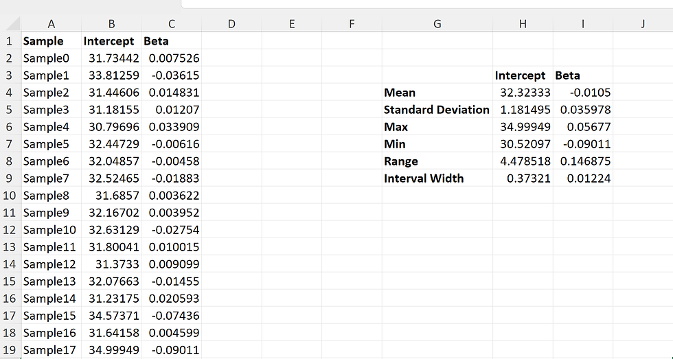
Lets get into a problem statement here, the objective of this problem is to estimate the value of a beta and intercept of a liner regressor, you need to also adjust the liner regression function with a error term, here in this case if are using a error between -2.0 to 2.0 . So our function is going to generate a set of random numbers between -2 to 2 as error and this will be added with the liner regression function, like that we need to create 50 such linear regression function, create an individual excel sheet for each of the linear regression function. Record the intercept , beta ,p-value, r value, r square, standard error, intercept error.
This is a pretty simple problem to think about, but for a beginner this could take a while to declutter, But the objective of such a problem is to give you a thread of what to expect from coding exercises with libraries . You can use chatgpt to extract full explanation of the code, I have included my own comments as well into the solution.
Documentation references,
# Importing necessary libraries
import random
import numpy as np
import pandas as pd
import os
from openpyxl import Workbook
from openpyxl.styles import Font, PatternFill
from scipy import stats

# Filepaths for dataset and output
filepath_for_dataset = "D:\datascience\data_set.xlsx"
filepath_for_output = "D:\datascience\data_with_index_2.xlsx"

# Generate random array for X values
# np.random.randint() function is used to generate random integers.
# Parameters:
#   - 20: Lower bound of the range (inclusive).
#   - 51: Upper bound of the range (exclusive).
#   - size=12: Specifies the size of the array to be generated, which is 12 in this case.
# This generates an array of 12 integers randomly sampled from the range [20, 51).
random_array_X = np.random.randint(20, 51, size=12)

# Generate random array for Y values
# Same logic as above, generating an array of 12 integers randomly sampled from the range [20, 51).
random_array_Y = np.random.randint(20, 51, size=12)


# Define array shape and range for floating-point numbers
# 'rows' and 'cols' define the shape of the 2D array to be generated.
# 'low' and 'high' specify the range of floating-point numbers to be generated.
rows = 50
cols = 12
low = -2.0
high = 2.0

# Generate random 2D array of floating-point numbers
# np.random.uniform() function is used to generate random floating-point numbers.
# Parameters:
#   - low: Lower bound of the range (inclusive).
#   - high: Upper bound of the range (exclusive).
#   - size=(rows, cols): Specifies the shape of the 2D array to be generated.
# This generates a 2D array of size (rows, cols) with floating-point numbers randomly sampled from the range [-2.0, 2.0).
random_2d_array = np.random.uniform(low, high, size=(rows, cols))

# Create DataFrame from arrays
# Creating a DataFrame named 'df' with two columns 'X' and 'Y' using random_array_X and random_array_Y.
# 'random_array_X' and 'random_array_Y' were generated previously.
df = pd.DataFrame({"X": random_array_X, "Y": random_array_Y})

# Generating column names for the second DataFrame 'df_2'.
# y = [f"Y_err_{x}" for x in range(50)] generates a list of column names from 'Y_err_0' to 'Y_err_49'.
'''This is a shorthand approach in python, what it does is creates a list internally and runs a loop ,
the loop results will be stored in that list. This technique enables you pack 4 lines of code into a single line.
Check this link for further reference, https://blog.finxter.com/python-one-line-for-loop-a-simple-tutorial/
'''


y = [f"Y_err_{x}" for x in range(50)]


# Creating 'df_2' DataFrame with random_2d_array reshaped into 12 rows and 50 columns, using column names from 'y'.
df_2 = pd.DataFrame(random_2d_array.reshape(12, 50), columns=y)

# Concatenate 'df' and 'df_2' DataFrames along columns (axis=1) to create a new DataFrame 'df_3'.
df_3 = pd.concat([df, df_2], axis=1)

# Adjust error value to Y
# Applying a lambda function to add values from 'df_3.iloc[:, 1]' (Y column) to each column in 'df_3.iloc[:, 2:]' (Y_err columns).
# This creates a DataFrame 'df_4' where each 'Y_err' value is adjusted by the corresponding 'Y' value.
'''Recall the lambda function , apply() is a method in pandas enable you to run some specific function to each cell in
panda dataframe, here we are using the lamda function to add individual values of one dataframe with other with lambda,
the lambda function is taking x as a parameter the x gets its value from the specific dataframe cell, This is a great approach
to do cell value manipulation in pandas.
'''
df_4 = df_3.iloc[:, 2:].apply(lambda x: x + df_3.iloc[:, 1], axis=0)

# Concatenate 'df' and 'df_4' DataFrames along columns (axis=1) to create a new DataFrame 'df_5'.
# This DataFrame includes both original 'X' and 'Y' columns from 'df', along with adjusted 'Y_err' columns from 'df_4'.
df_5 = pd.concat([df, df_4], axis=1)

rs = []
for x in range(2, df_5.shape[1]):
    res = stats.linregress(df_5.iloc[:, 0], df_5.iloc[:, x])
    rs_ = rs.append({
        "intercept": res.intercept,
        "beta": res.slope,
        "rvalue": res.rvalue,
        "pvalue": res.pvalue,
        "r_sqr": res.rvalue ** 2,
        "standard_error": res.intercept_stderr,
        "intercept_stderr": res.intercept_stderr
    })
aa = pd.DataFrame(rs)

# Write DataFrame to Excel
with pd.ExcelWriter(filepath_for_dataset, engine='xlsxwriter') as writer:
    df_5.to_excel(writer, sheet_name='Data', index=False)

# Create a new Excel workbook
workbook = Workbook()
bold_font = Font(bold=True)
highlight_color = "FFFF00"
highlight_fill = PatternFill(start_color=highlight_color,
                             end_color=highlight_color,
                             fill_type="solid")


# Create a new Excel workbook
workbook = Workbook()
# Make the text in cell A1 bold
bold_font = Font(bold=True)
# Define the background color you want to use for highlighting
highlight_color = "FFFF00"  # Yellow color, you can change it as needed

# Create a pattern fill with the specified color
highlight_fill = PatternFill(start_color=highlight_color,
                             end_color=highlight_color,
                             fill_type="solid")

sheet_coeff = workbook.create_sheet(title="Coefficients")
sheet_coeff[f"A{1}"] = str("Sample")
sheet_coeff[f"B{1}"] = str("Intercept")
sheet_coeff[f"C{1}"]= str("Beta")
sheet_coeff[f"A{1}"].font = bold_font
sheet_coeff[f"B{1}"].font = bold_font
sheet_coeff[f"C{1}"].font= bold_font

#metrics
sheet_coeff[f"G{4}"] = str("Mean")
sheet_coeff[f"G{5}"] = str("Standard Deviation")
sheet_coeff[f"G{6}"]= str("Max")
sheet_coeff[f"G{7}"] = str("Min")
sheet_coeff[f"G{8}"] = str("Range")
sheet_coeff[f"G{9}"]= str("Interval Width")
sheet_coeff[f"H{3}"] = str("Intercept")
sheet_coeff[f"I{3}"] = str("Beta")
sheet_coeff[f"H{3}"].font = bold_font
sheet_coeff[f"I{3}"].font = bold_font

sheet_coeff[f"H{4}"] = aa.iloc[:,:2].mean()[0]
sheet_coeff[f"H{5}"] = aa.iloc[:,:2].std()[0]
sheet_coeff[f"H{6}"]= aa.iloc[:,:2].max()[0]
sheet_coeff[f"H{7}"] = aa.iloc[:,:2].min()[0]
sheet_coeff[f"H{8}"] = (aa.iloc[:,:2].max()[0]-aa.iloc[:,:2].min()[0])
sheet_coeff[f"H{9}"]= (aa.iloc[:,:2].max()[0]-aa.iloc[:,:2].min()[0])/df_5.shape[0]

sheet_coeff[f"G{4}"].font = bold_font
sheet_coeff[f"G{5}"].font = bold_font
sheet_coeff[f"G{6}"].font= bold_font
sheet_coeff[f"G{7}"].font = bold_font
sheet_coeff[f"G{8}"].font = bold_font
sheet_coeff[f"G{9}"].font= bold_font


sheet_coeff[f"G{4}"] = str("Mean")
sheet_coeff[f"G{5}"] = str("Standard Deviation")
sheet_coeff[f"G{6}"]= str("Max")
sheet_coeff[f"G{7}"] = str("Min")
sheet_coeff[f"G{8}"] = str("Range")
sheet_coeff[f"G{9}"]= str("Interval Width")

sheet_coeff[f"I{4}"] = aa.iloc[:,:2].mean()[1]
sheet_coeff[f"I{5}"] = aa.iloc[:,:2].std()[1]
sheet_coeff[f"I{6}"]= aa.iloc[:,:2].max()[1]
sheet_coeff[f"I{7}"] = aa.iloc[:,:2].min()[1]
sheet_coeff[f"I{8}"] = (aa.iloc[:,:2].max()[1]-aa.iloc[:,:2].min()[1])
sheet_coeff[f"I{9}"]= (aa.iloc[:,:2].max()[1]-aa.iloc[:,:2].min()[1])/df_5.shape[0]

sheet_coeff[f"G{4}"].font = bold_font
sheet_coeff[f"G{5}"].font = bold_font
sheet_coeff[f"G{6}"].font= bold_font
sheet_coeff[f"G{7}"].font = bold_font
sheet_coeff[f"G{8}"].font = bold_font
sheet_coeff[f"G{9}"].font= bold_font


# Loop over the index of the DataFrame
for index in aa.index:
    sheet_coeff[f"A{index+2}"]= f"Sample{index}"
    sheet_coeff[f"B{index+2}"] = aa.loc[index][0]
    sheet_coeff[f"C{index+2}"] = aa.loc[index][1]


# Loop over the index of the DataFrame
for index in aa.index:
    # Create a new sheet for each index
    sheet = workbook.create_sheet(title=f"Y_{index}")
    sheet[f"A{1}"] = str("X")
    sheet[f"B{1}"] = str("Y")
    sheet[f"C{1}"] = str("Y_error")
    sheet[f"A{1}"].font = bold_font
    sheet[f"B{1}"].font = bold_font
    sheet[f"C{1}"].font = bold_font

    for count in range(df.shape[0]):
        sheet[f"A{count+2}"] = df_5.X[count]
        sheet[f"B{count+2}"] = df_5.Y[count]
        sheet[f"C{count+2}"] = df_5.loc[count][index+2]


    for count in range(aa.shape[1]):
        sheet[f"E{count+1}"] = str.upper(aa.columns[count])
        sheet[f"E{count+1}"].font=bold_font
        sheet[f"E{count+1}"].fill=highlight_fill
        sheet[f"F{count+1}"] = aa.loc[index][count]


# Remove the default sheet created by openpyxl
workbook.remove(workbook.active)

# Save the workbook
workbook.save(filename=filepath_for_output)
Comments